Guided Super Resolution as Pixel-to-Pixel Transformation Paper Review

In this blog post I will try to explain what I have understand from the paper Guided Super Resolution as Pixel-to-Pixel Transformation which I hope it helps for who is interested. As a matter of fact, all the information is gathered from the paper itself otherwise it will be indicated.

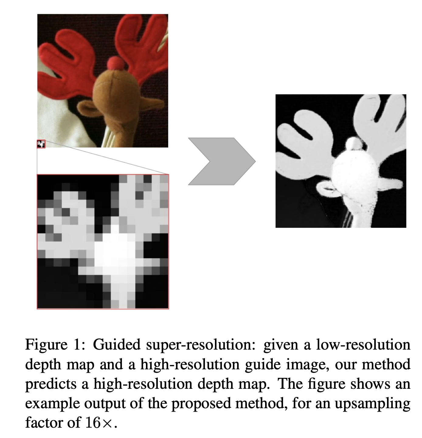
First let’s start with some definition of the problem. The task of Guided Super Resolution can be defined as a unifying framework for several computer vision tasks where the inputs are

• a low resolution source image of some target quantity
• a high resolution guide image from different domain and the target output is the high resolution version of the source image.

There are mainly 3 entities of the problem:

Guide image, source image and the target image.

Maybe you are asking what is the objective there? If we have the high-resolution guide why we are bothering ourselves to transform the source image. The objective relies on the domain difference. For example generally robots have two different cameras to construct vision with depth perception. First camera is a conventional camera that gathers RGB image, the second is time-of-flight camera or laser scanner which collects the depth information. But mostly the second camera has a very low resolution compared to the conventional camera. The objective is to transform this low-res image to a high-res image with the help of the guide image. We are trying to transfer high frequency details to the upsampled image of the source to obtain a sharp, high resolution version of it with the depth information.

Related Work

The starting point of Guided Super Resolution task is definitely bilateral filter. Bilateral Filter is a non-linear edge preserving filter that is widely used in image processing for noise reduction. The simple idea that relies behind this filter is the necessary information for a pixel value can be modeled as weighted average of the local neighborhood information.

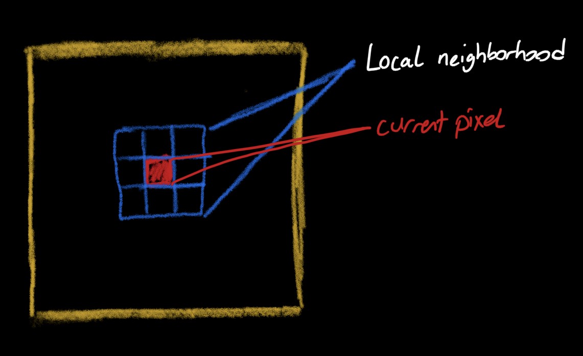
Bilateral filter is a conventional technique that gets a pixel and returns the weighted average of local neighborhood pixels. It is used for edge preserving, noise reduction and also for super-resolution. Low-resolution image upsampled to a higher one and than this image goes through Bilateral Filter to get smoother. Actually, Bilateral Filter is generalized version of the Guided Filters.

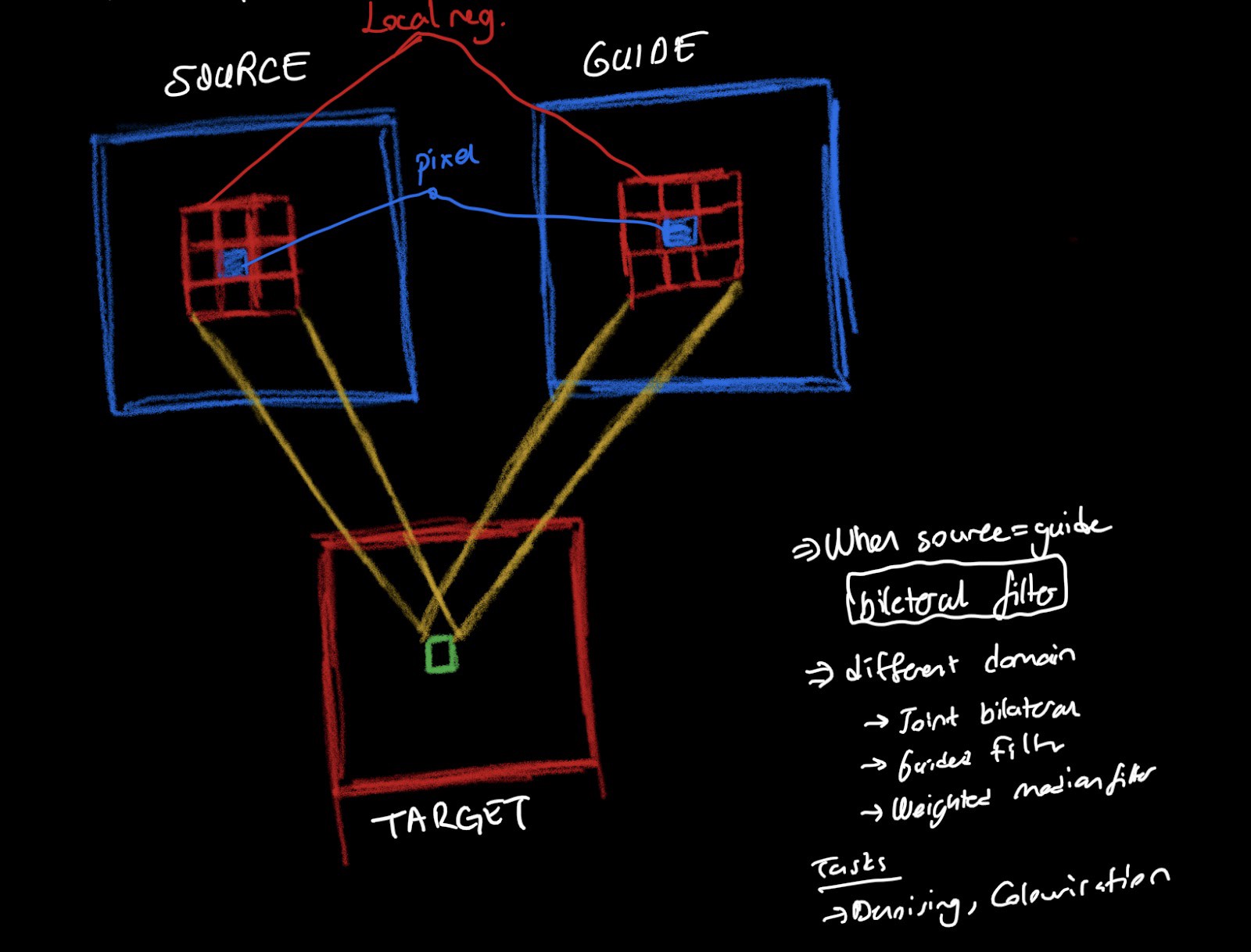
Guided Filter is a framework that gets two images -one as a guide and the other one is the source- and returns the combination of the weighted averages for that pixel in both source and the guide image. It is used also for denoising and colorisation.

In the paper we dealt with not Guided Filter but Guided Super-Resolution task. It is the same as Guided Filters except we have the source at a lower resolution than the guide. Guided Super Resolution task extends the problem by adding super resolution which means transforming the source from lower to a higher resolution. This methods could be divided into two parts, first is local methods as for the Bilateral and Guided Filters, second is the global methods that formulate upsampling task as a global energy minimization.

The local methods consist of two step, first upsampling the source image to the higher resolution, then enhancing by the high-res guide. Global methods, instead trying to find a function that gets the source image and converts it to a high resolution target as good as possible. We define a loss function that aligned with the source, and trying to minimize this loss during the process.

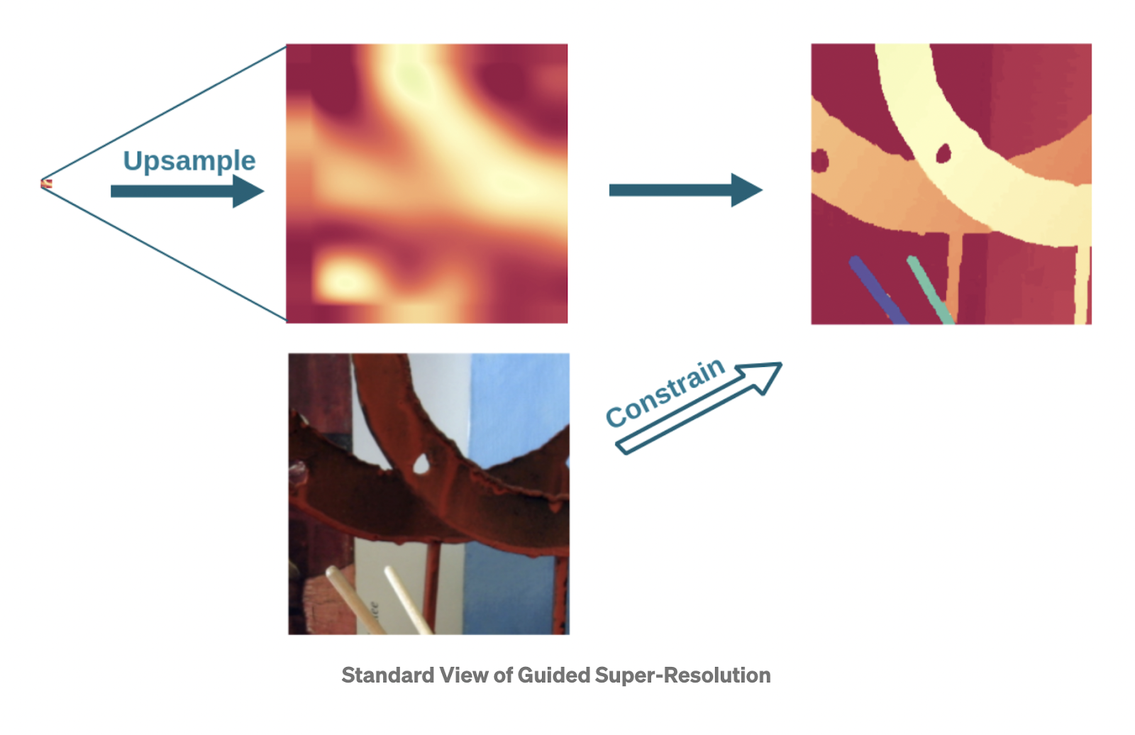
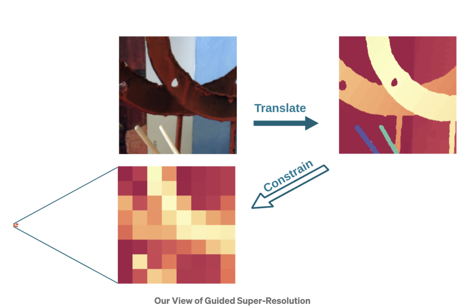
The Classical Approach to this task to formulate the task as an inverse problem: The source is understood as the result of downsampling the target image and the objective is to undo that operation by utilising the guide image to constrain the solution.

Architecture and Implementation

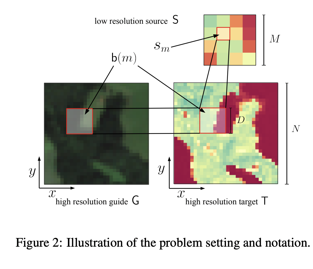
We have three different images : S(MxM) is the source, G(NxN) is the guide, and T(NxN) is the target image. Because the source is at a lower resolution, we have mapped DxD pixels of the guide or target to one pixel of the source. While mapping we are averaging the pixel value of the DxD pixels and these group of the pixels are denoted by b(m).

Now we are getting to the most important part of the paper: creating the loss function step by step. First, lets set the problem and the objective:

We can formulate the problem as : Finding a function that

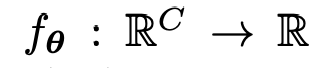
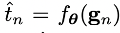
gets the whole guide pixels and returns the target pixels where target pixels are consistent with the source.

As the first step of the Loss function we can start by :

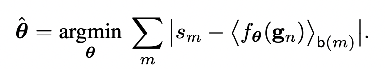
But there is a problem with that loss function, it is obviously ill-posed because we are downsampling the target function by averaging the DxD pixels, and there will be many solutions for that problem. Additionally, as indicated in the paper, for a given S, T, and G a perfect solution could be found by choosing a sufficiently complex function. So, we can solve this issue by regularizing with the l2 regularization our parameters. Our loss function will be :

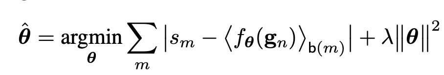
When we are looking this loss, we can easily see there is one-to-one relationships regardless of the locations. So, we can give the location information of the pixel as an input, by doing this we allow the function to take into account the location at the mapping stage.

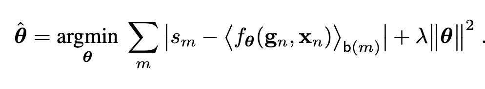
Now as a last problem, we are pushing not only guide pixel function, but also spatial function to be simple functions because of the same amount of regularization λ. We can separate the architecture into two parts: one for the pixel information and the other is the spatial information then combining them again.

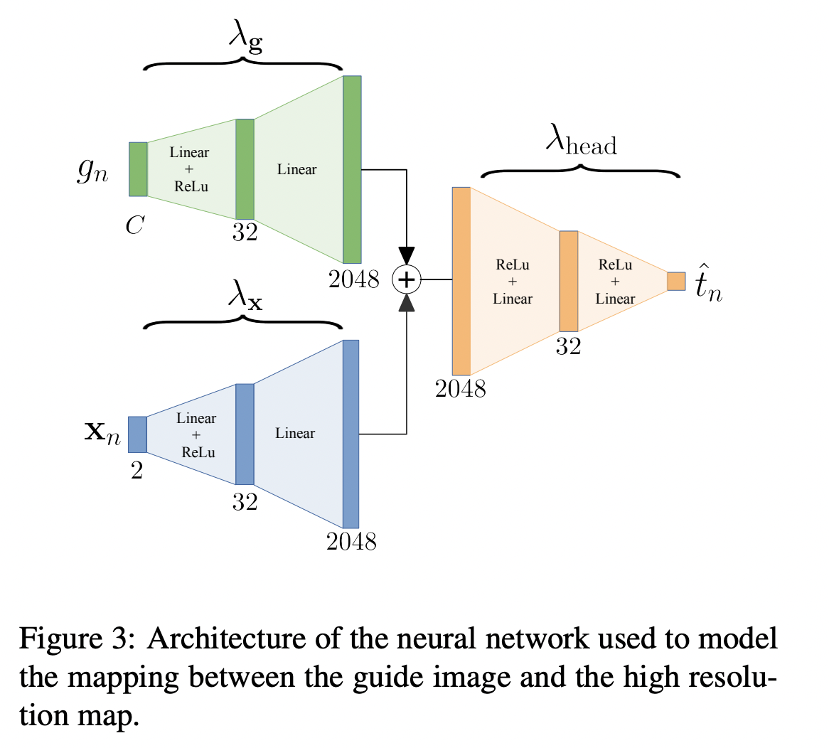
By this architecture, we have 3 different regularization coefficients: λg, λx and λhead. By this architecture we can obtain sharp and crisp target images.

For optimisation, classical stochastic gradient descent could be used. The architecture can be implemented by Convolutional neural nets by any deep learning framework. Author’s implementation with PyTorch could be found at https://github.com/prs-eth/PixTransform.

I will finish by an important remark for the method. The method is unsupervised, which means you do not need other images than just Source, Guide and Target images. But you cannot use the same function for a different image. For every new image you should train the parameters again. One may ask, where is the neural network then, if we cannot use it for other cases? Actually the tricky part is here, the trained network generalize not the images, but pixels, we obtain a generalized function for every pixel of the image. As the title of the paper shows : it is Pixel-to-Pixel transformation.

For the results, I have run the code provided by the authors:

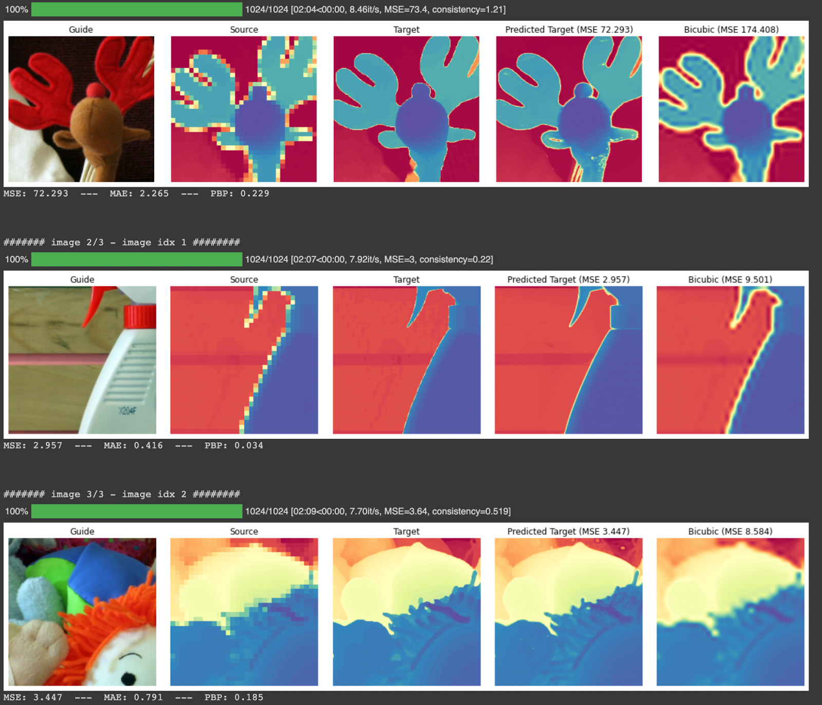
The results of the experiment could be summarized as:

• Paper results are reproduced, because it is an unsupervised technique we can use it for other datasets
• Because training and prediction must be done in the same stage, it becomes slow for inference. Thus it cannot be used for a streaming process.
• For the high upsampling factors like 32x, the training is much longer and produced results are not quite good.
• In 2022, there is proposed another solution by the same author as Learning Graph Regularization for Guided Super Resolution which does a better job with a bunch of data.

Thank you for reading!!